[ML] PCA 主成份分析
在上一篇的文章中,檸檬爸首先介紹如何使用 Python 與 Numpy 函式庫將想要分析的圖片載入多維的空間中,接下來就是需要開始分析這些圖片,假設一開始並不知道這些圖片的標籤的時候,我們沒有辦法執行分類的訓練。本篇想要介紹一下 Principle Component Analysis, PCA 主成份分析這一個方法背後的數學理論與物理意義,參考的是台大資工系林軒田教授的講義,在林教授的講解過程中,PCA 其實是 Auto-Encoder 中的一個線性特例,如果從 Auto-Encoder 的角度來看 PCA 的話可以更加了解 PCA 主成份分析的物理意義!
可以描述成以下的數學式,輸入是維度為 一般情況的 Auto-Encoder
![Rendered by QuickLaTeX.com d](https://myoceane.fr/wp-content/ql-cache/quicklatex.com-4e8716946f6a868f015e0d62f28bc540_l3.png)
![Rendered by QuickLaTeX.com \textbf{x}](https://myoceane.fr/wp-content/ql-cache/quicklatex.com-27a2f7ab513a764b16fc08c9df21cf7a_l3.png)
![Rendered by QuickLaTeX.com \tilde{d}](https://myoceane.fr/wp-content/ql-cache/quicklatex.com-329096e09eff5f7afa800b67eb62a5fb_l3.png)
![Rendered by QuickLaTeX.com h_i(\textbf{x})](https://myoceane.fr/wp-content/ql-cache/quicklatex.com-17f23211e661dd75ac0d9b4d9d3daf41_l3.png)
![Rendered by QuickLaTeX.com d](https://myoceane.fr/wp-content/ql-cache/quicklatex.com-4e8716946f6a868f015e0d62f28bc540_l3.png)
(1)
線性的情況則可以描述成以下的數學式,輸入是維度為 線性的 Auto-Encoder
![Rendered by QuickLaTeX.com d](https://myoceane.fr/wp-content/ql-cache/quicklatex.com-4e8716946f6a868f015e0d62f28bc540_l3.png)
![Rendered by QuickLaTeX.com \textbf{x}](https://myoceane.fr/wp-content/ql-cache/quicklatex.com-27a2f7ab513a764b16fc08c9df21cf7a_l3.png)
![Rendered by QuickLaTeX.com \tilde{d}](https://myoceane.fr/wp-content/ql-cache/quicklatex.com-329096e09eff5f7afa800b67eb62a5fb_l3.png)
![Rendered by QuickLaTeX.com h_i(\textbf{x})](https://myoceane.fr/wp-content/ql-cache/quicklatex.com-17f23211e661dd75ac0d9b4d9d3daf41_l3.png)
![Rendered by QuickLaTeX.com d](https://myoceane.fr/wp-content/ql-cache/quicklatex.com-4e8716946f6a868f015e0d62f28bc540_l3.png)
(2)
![Rendered by QuickLaTeX.com w^{(2)}_{ji}=w^{(1)}_{ij}=w_{ij}](https://myoceane.fr/wp-content/ql-cache/quicklatex.com-2a9b69b3e27a620856b27142492b3bac_l3.png)
![Rendered by QuickLaTeX.com W=[w_{ij}]](https://myoceane.fr/wp-content/ql-cache/quicklatex.com-7a7dedafd7676abf00c4c8314f1d0117_l3.png)
![Rendered by QuickLaTeX.com d\times\tilde{d}](https://myoceane.fr/wp-content/ql-cache/quicklatex.com-4f55beb012e301441d6b27fef4f55e9a_l3.png)
![Rendered by QuickLaTeX.com \tilde{d} < d](https://myoceane.fr/wp-content/ql-cache/quicklatex.com-d90d1f3a55dfe923e74d1f833c5a71da_l3.png)
(3)
首先我們利用 eigen-decompose 的技術將 物理意義
![Rendered by QuickLaTeX.com WW^T](https://myoceane.fr/wp-content/ql-cache/quicklatex.com-a98b34f79b82d639c703fbc6ec6e1625_l3.png)
![Rendered by QuickLaTeX.com V](https://myoceane.fr/wp-content/ql-cache/quicklatex.com-63ada879859a9e41fd935f035b7313bc_l3.png)
![Rendered by QuickLaTeX.com d\times d](https://myoceane.fr/wp-content/ql-cache/quicklatex.com-67c75e302037c3e64e5f3022c8f0babe_l3.png)
![Rendered by QuickLaTeX.com VV^T = V^TV = I_d](https://myoceane.fr/wp-content/ql-cache/quicklatex.com-acf2f4f1f4186f512c7808efea719b83_l3.png)
![Rendered by QuickLaTeX.com \Gamma](https://myoceane.fr/wp-content/ql-cache/quicklatex.com-4f420945e64069f30b66c3d17e2f98ac_l3.png)
![Rendered by QuickLaTeX.com \leq\tilde{d}](https://myoceane.fr/wp-content/ql-cache/quicklatex.com-51e1e354f6fc2278e3d37a9f117f5109_l3.png)
![Rendered by QuickLaTeX.com W \in R^{d\times\tilde{d}}](https://myoceane.fr/wp-content/ql-cache/quicklatex.com-39d5e689e69c94c7a3bb03bc0df8e33c_l3.png)
(4)
所以線性 Auto-Encoder 的物理意義就是:
- 先利用一個 orthonormal 的基礎向量集合 V 將 x 向量轉置到另外一個向量空間 (Vector Space)
- 將一部分維度放大縮小,另外一部分維度設成 0
- 再利用同一組基礎向量集合將處理過後的向量轉回原本的向量空間
![Rendered by QuickLaTeX.com \Gamma = I](https://myoceane.fr/wp-content/ql-cache/quicklatex.com-0c6c9abcb8953e0add0c16288cb429b2_l3.png)
(5)
有了以上對 Auto-Encoder 的描述,我們可以架構我們的問題為:找出一個最佳化的矩陣 Problem Formulation 問題表述
![Rendered by QuickLaTeX.com W](https://myoceane.fr/wp-content/ql-cache/quicklatex.com-4caed22919a1780df1b6310b338b904e_l3.png)
![Rendered by QuickLaTeX.com V, \Gamma](https://myoceane.fr/wp-content/ql-cache/quicklatex.com-aa5bc9a6982b1d56d251b67e66cec1ae_l3.png)
![Rendered by QuickLaTeX.com h(\textbf{x})](https://myoceane.fr/wp-content/ql-cache/quicklatex.com-a7c73c15a6b74b6df5341df7e87e095b_l3.png)
![Rendered by QuickLaTeX.com E_{\text{in}}(\textbf{h})](https://myoceane.fr/wp-content/ql-cache/quicklatex.com-61b09b635a96817e8447e0136ab65e26_l3.png)
(6)
求解 W
以下我們 go through 一遍講義中的線性代數證明,也就是求解以下的最佳化問題:
(7)
因為使用 orthonormal 的向量集合轉置到另外一個向量空間並不會影響長度,所以我們將問題簡化,
(8)
![Rendered by QuickLaTeX.com (I-\Gamma)](https://myoceane.fr/wp-content/ql-cache/quicklatex.com-6170d8274cb9163298071c5df1c8028a_l3.png)
![Rendered by QuickLaTeX.com \Gamma = \begin{bmatrix} I_{\tilde{d}} & 0\\ 0 & 0 \end{bmatrix}](https://myoceane.fr/wp-content/ql-cache/quicklatex.com-e33d4960b84945714ffd1d51f4a62bac_l3.png)
(9)
![Rendered by QuickLaTeX.com \tilde{d} = 1](https://myoceane.fr/wp-content/ql-cache/quicklatex.com-7da7d606603ef48bd02af01998f1650e_l3.png)
![Rendered by QuickLaTeX.com \textbf{v}](https://myoceane.fr/wp-content/ql-cache/quicklatex.com-9951ed4030dcb53d250cd1e29f000357_l3.png)
![Rendered by QuickLaTeX.com \textbf{v}^T\textbf{v} = 1](https://myoceane.fr/wp-content/ql-cache/quicklatex.com-a437afefeb158252ffafc376695c0473_l3.png)
(10)
![Rendered by QuickLaTeX.com \sum^{N}_{n=1}\textbf{x}_n\textbf{x}^T_n\textbf{v} = X^T X \textbf{v}= \lambda\textbf{v}](https://myoceane.fr/wp-content/ql-cache/quicklatex.com-cd7a2d0cc6ddbf34cc6ac24e08cbd0aa_l3.png)
![Rendered by QuickLaTeX.com \tilde{d}=1](https://myoceane.fr/wp-content/ql-cache/quicklatex.com-50c8ff3bbe0dbdc73af49f6dcc6f0a34_l3.png)
![Rendered by QuickLaTeX.com X^TX](https://myoceane.fr/wp-content/ql-cache/quicklatex.com-45ae6e224610b89cbcb8217f0b82df04_l3.png)
![Rendered by QuickLaTeX.com \textbf{v}](https://myoceane.fr/wp-content/ql-cache/quicklatex.com-9951ed4030dcb53d250cd1e29f000357_l3.png)
![Rendered by QuickLaTeX.com \tilde{d} \leq d](https://myoceane.fr/wp-content/ql-cache/quicklatex.com-06d42127c4a782d7620f32e6692ff86e_l3.png)
![Rendered by QuickLaTeX.com W=\{w_j\}=\{v_j\}^{\tilde{d}}_{j=1}](https://myoceane.fr/wp-content/ql-cache/quicklatex.com-d0731739406dcb4bc063b724b6bdd828_l3.png)
![Rendered by QuickLaTeX.com X^TX](https://myoceane.fr/wp-content/ql-cache/quicklatex.com-45ae6e224610b89cbcb8217f0b82df04_l3.png)
![Rendered by QuickLaTeX.com \tilde{d}](https://myoceane.fr/wp-content/ql-cache/quicklatex.com-329096e09eff5f7afa800b67eb62a5fb_l3.png)
PCA 與 Auto-Encoder 的差異
其實 PCA 與 Auto-Encoder 在處理的問題還是有一點差異的,Auto-Encoder 是在處理最大化長度的問題,而 PCA 則是在處理最大化變異數的問題,但是其實兩個問題的本質是一樣的。
(11)
PCA 在 Clustering 的應用實例
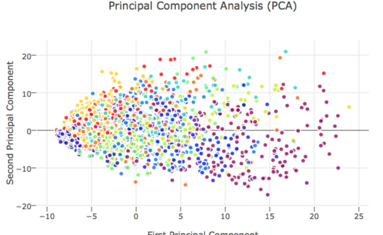
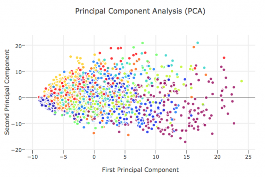
在以下連結中,作者使用 scikit-Learn 中的 PCA 主成份分析工具分析 MNIST 的圖片:
原本資料維度為 28 * 28 = 784 維,本篇作者展示將資料降維成 40 維一樣可以保持資料之間的差異性保持住,這邊值得一提的作者執行 PCA 之前有用
from sklearn.preprocessing import StandardScaler
X_std = StandardScaler().fit_transform(X)
先將資料去平均值與正規化,其實就是式子 (11) 在做的事情,取最大變異的兩個維度,可以得到以下的結果,結果顯示利用 PCA 降成兩個維度在做機器學習的效果可能部會太好,這邊可能要考慮使用一些非線性的分類方法,例如 t-SNE 等等!
![](https://myoceane.fr/wp-content/uploads/2020/04/螢幕快照-2020-04-24-下午10.27.30-1024x684.png)